Flight Numbers: Determining if 2020 offered a large enough sample size of stats
October 26, 2020 by Aaron Howard in Analysis
The 2020 season has had a relative dearth of tournaments. While the Pro Tour got its full slate in, there was no National Tour, no West Coast swing, and no World Championship. This small number of events got me thinking about sample size, and whether or not players’ statistics, specifically the widely cited UDisc stats, from this year are “reliable.”
This is an age old question in sports. When is a hot start to a season no longer a fluke? Or when is a slump no longer a slump and indicative of injury, physical decline, or aging? If sample size is small (e.g. only a few holes or maybe even tournaments), there is a lot of noise or randomness in outcomes (I can hit almost any green once, right?). It’s not until we have a lot of data that true talent is represented.
This question was first addressed in baseball, of course, as is the case with most sports analytics questions like these. For example, sabermetricians wanted to know how many at bats it takes for on-base percentage to stabilize, and teams eventually realized that they could use this type of information to decide when to bring players up to the majors or whether or not to sign a player to a contract extension..
But what does this look like in disc golf? Well, the most direct application would be to determine how many holes it takes for circle one in regulation, or fairway hits, or whatever stat you are interested in, to stabilize.
What does “stabilize” mean? It can mean a lot of things, but the most intriguing is: when are differences between players’ stats more representative of true skill than randomness? Or in the context of 2020, can we trust the stats from this year, or were there too few events for them to be reliable?
Methods
If you are not interested in the nitty gritty details of how I calculated when UDisc stats stabilize, then skip this part and just read the results in the next section.
My methods are based on those developed for baseball and explained fairly in depth here and here. I used all of the UDisc data from 2019 for this analysis. I didn’t use 2020 because, as I said above, it’s a weird year and I wanted to consider data that are widely applicable.
To start, I used the binomial distribution to calculate the expected random variation found in each statistic.1 The binomial distribution is one that is used to model events with two outcomes, such as a coin flip. The variation in a coin flip is random. You expect half of the flips to be heads and half to be tails, but they aren’t always perfectly 50/50. That random variation in coin flips can be calculated using the binomial distribution. A coin flip distribution makes sense for UDisc stats because each occurrence of a statistical category is measured at a yes/no (heads or tails) level. One hits the green on a hole or one doesn’t. One makes the circle one putt or one doesn’t.
Then, I calculated the observed variance, or how much variance we see in each statistic. This observed variance is composed of two things: the influence of luck (random variance) and skill (true variance). Knowing this, I subtracted out the random variance, which gives us a measure of true statistical variance.
Finally, I went back to the binomial distribution and calculated the number of holes it takes for the true and random variances to be equal. This is when statistics represent true skill as much as luck.
Results
The number of holes at which each statistic stabilizes is shown in the plot below. There are a few big picture patterns to notice: C1R and C2R stabilize very quickly, after just a few rounds. For MPO, putting statistics take twice as long. It takes about an entire four round event for MPO C1 and C2 putting values to become reliable.
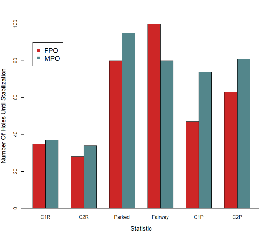
What do these differences mean? They show us that the ratio of random variance to true variance (skill) is much higher in the putting statistics, and it takes longer (more holes) for the true variance to equal the random variance. Let us be clear in the interpretation here because it is a bit nuanced. This doesn’t mean there is less skill involved in putting than hitting greens, but it does mean that the variation in true skill is less for putting.
This difference in the ratio of true to random variation is best exemplified with the results of a statistic I didn’t include in the plot: throw-in rate.2 It takes approximately 760 holes for throw-in rates to stabilize for MPO. That is because there is a lot of random noise, relative to skill, in this statistic. This is an extreme example of what I discussed above with putting. There is skill in making throw-ins, but there is also a great deal of luck, as we can all relate to.
In fact, there is more luck to throw-ins than skill. The true to random variance ratio for this statistic is below 1, 0.68 to be precise. This same ratio for C1R is about 15 and for C1X putting it is 7.
This isn’t as true for FPO. While putting does take longer than circles in regulation stats to stabilize, they do not take nearly as long as MPO. Again, this means there is more true skill variance on the green for FPO than MPO. It also means there are more strokes to gain putting for FPO than MPO, and that can help explain why a player like Heather Young, who is in the bottom half of the field in C1R but sitting at number 1 in C1X, can still compete.
Conclusions
Before bringing these results back to 2020, I would like to address an application of these methods to baseball that I mentioned in the introduction. Teams can use these methods to interpret a minor league player’s “cup of coffee” or whether or not to offer contracts.3 But you may be asking yourself, why does baseball use “when true variance equals random variance” as their cutoff point? Well, as I briefly mentioned, it is a tipping point. It is when statistics start to become more representative of skill than luck. However, it is also the cutoff point because of a practical consideration – there is a lot of noise in baseball statistics. For example, on-base percentage does not start to stabilize until over 300 plate appearances, which takes on average a half of a season to accumulate!
Fortunately for disc golf, most of our stats appear to stabilize much faster. So, when applying this concept to disc golf, we can be a lot more stringent. For example, if manufacturers are trying to assess players for sponsorship, I think it would be prudent for them to set a higher cutoff point, say when true variance is 3x larger than random variance, for the green in regulation stats. For C2R, this would equate to about 108 holes, or only two three-round events. This would significantly reduce the risk of sponsoring a player that simply had a great round or two, while not requiring an unrealistically large number of events.
Finally, let’s bring these results back to the 2020 season, the initial reason I started on the project. In short, we have plenty of data from this year to feel confident about most UDisc stats’ meaning. Even if we only considered the DGPT events, we would have more than enough data for all but throw-ins.
So, dig into those UDisc stats with confidence, and use them to come to your own conclusions about things like Player of the Year awards. I know I will!
I calculated the random variance using this equation: variance = p*(1-p) / n, where p is the probability of the stat of interest (e.g., C1R), and n is the sample size (number of holes). ↩
I didn’t include it on the plot because it is about an order of magnitude higher than the other stats values, which would throw off the y-axis scaling and render the plot unreadable. ↩
The application of these stabilization methods in this context actually requires an additional computational step called regression to the mean, but this article is long enough as is, so I will save it for the next one. ↩